TABLE/目录

注：后半部分为我的内容，如果你感觉难以跟上前半段英文教程，你也可以直接跳到我的实现部分并copy代码，但我并不建议这么做。
注：在真正开始之前，你可能需要把tensorflow安装好。然而相比于安装pytorch，tensorflow的安装实在是个大工程。
本文前半部分转载于Image classification from scratch
Author: fchollet
Date created: 2020/04/27
Last modified: 2020/04/28
Description: Training an image classifier from scratch on the Kaggle Cats vs Dogs dataset.

Introduction

This example shows how to do image classification from scratch, starting from JPEG image files on disk, without leveraging pre-trained weights or a pre-made Keras Application model. We demonstrate the workflow on the Kaggle Cats vs Dogs binary classification dataset.

We use the image_dataset_from_directory utility to generate the datasets, and we use Keras image preprocessing layers for image standardization and data augmentation.

Setup

import tensorflow as tf
from tensorflow import keras
from tensorflow.keras import layers

Load the data: the Cats vs Dogs dataset

Raw data download

First, let’s download the 786M ZIP archive of the raw data:

$ curl -O https://download.microsoft.com/download/3/E/1/3E1C3F21-ECDB-4869-8368-6DEBA77B919F/kagglecatsanddogs_3367a.zip

$ unzip -q kagglecatsanddogs_3367a.zip

Now we have a PetImages folder which contain two subfolders, Cat and Dog. Each subfolder contains image files for each category.

$ ls
Cat/  Dog/

Filter out corrupted images

When working with lots of real-world image data, corrupted images are a common occurence. Let’s filter out badly-encoded images that do not feature the string “JFIF” in their header.

import os

num_skipped = 0
for folder_name in ("Cat", "Dog"):
    folder_path = os.path.join("PetImages", folder_name)
    for fname in os.listdir(folder_path):
        fpath = os.path.join(folder_path, fname)
        try:
            fobj = open(fpath, "rb")
            is_jfif = tf.compat.as_bytes("JFIF") in fobj.peek(10)
        finally:
            fobj.close()

        if not is_jfif:
            num_skipped += 1
            # Delete corrupted image
            os.remove(fpath)

print("Deleted %d images" % num_skipped)

Deleted 1590 images

Generate a Dataset

image_size = (180, 180)
batch_size = 32

train_ds = tf.keras.preprocessing.image_dataset_from_directory(
    "PetImages",
    validation_split=0.2,
    subset="training",
    seed=1337,
    image_size=image_size,
    batch_size=batch_size,
)
val_ds = tf.keras.preprocessing.image_dataset_from_directory(
    "PetImages",
    validation_split=0.2,
    subset="validation",
    seed=1337,
    image_size=image_size,
    batch_size=batch_size,
)

Found 23410 files belonging to 2 classes.
Using 18728 files for training.
Found 23410 files belonging to 2 classes.
Using 4682 files for validation.

Visualize the data

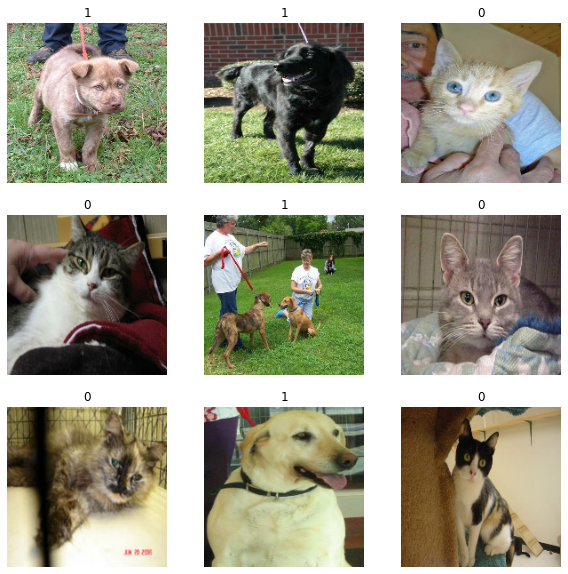
Here are the first 9 images in the training dataset. As you can see, label 1 is “dog” and label 0 is “cat”.

import matplotlib.pyplot as plt

plt.figure(figsize=(10, 10))
for images, labels in train_ds.take(1):
    for i in range(9):
        ax = plt.subplot(3, 3, i + 1)
        plt.imshow(images[i].numpy().astype("uint8"))
        plt.title(int(labels[i]))
        plt.axis("off")

Using image data augmentation

When you don’t have a large image dataset, it’s a good practice to artificially introduce sample diversity by applying random yet realistic transformations to the training images, such as random horizontal flipping or small random rotations. This helps expose the model to different aspects of the training data while slowing down overfitting.

data_augmentation = keras.Sequential(
    [
        layers.RandomFlip("horizontal"),
        layers.RandomRotation(0.1),
    ]
)

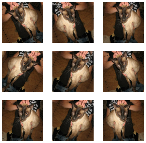
Let’s visualize what the augmented samples look like, by applying data_augmentation repeatedly to the first image in the dataset:

plt.figure(figsize=(10, 10))
for images, _ in train_ds.take(1):
    for i in range(9):
        augmented_images = data_augmentation(images)
        ax = plt.subplot(3, 3, i + 1)
        plt.imshow(augmented_images[0].numpy().astype("uint8"))
        plt.axis("off")

Standardizing the data

Our image are already in a standard size (180x180), as they are being yielded as contiguous float32 batches by our dataset. However, their RGB channel values are in the [0, 255] range. This is not ideal for a neural network; in general you should seek to make your input values small. Here, we will standardize values to be in the [0, 1] by using a Rescaling layer at the start of our model.

Two options to preprocess the data

There are two ways you could be using the data_augmentation preprocessor:

Option 1: Make it part of the model, like this:

inputs = keras.Input(shape=input_shape)
x = data_augmentation(inputs)
x = layers.Rescaling(1./255)(x)
...  # Rest of the model

With this option, your data augmentation will happen on device, synchronously with the rest of the model execution, meaning that it will benefit from GPU acceleration.

Note that data augmentation is inactive at test time, so the input samples will only be augmented during fit(), not when calling evaluate() or predict().

If you’re training on GPU, this is the better option.

Option 2: apply it to the dataset, so as to obtain a dataset that yields batches of augmented images, like this:

augmented_train_ds = train_ds.map(
  lambda x, y: (data_augmentation(x, training=True), y))

With this option, your data augmentation will happen on CPU, asynchronously, and will be buffered before going into the model.

If you’re training on CPU, this is the better option, since it makes data augmentation asynchronous and non-blocking.

In our case, we’ll go with the first option.

Configure the dataset for performance

Let’s make sure to use buffered prefetching so we can yield data from disk without having I/O becoming blocking:

train_ds = train_ds.prefetch(buffer_size=32)
val_ds = val_ds.prefetch(buffer_size=32)

Build a model

We’ll build a small version of the Xception network. We haven’t particularly tried to optimize the architecture; if you want to do a systematic search for the best model configuration, consider using KerasTuner.

Note that:

We start the model with the data_augmentation preprocessor, followed by a Rescaling layer.
We include a Dropout layer before the final classification layer.

def make_model(input_shape, num_classes):
    inputs = keras.Input(shape=input_shape)
    # Image augmentation block
    x = data_augmentation(inputs)

    # Entry block
    x = layers.Rescaling(1.0 / 255)(x)
    x = layers.Conv2D(32, 3, strides=2, padding="same")(x)
    x = layers.BatchNormalization()(x)
    x = layers.Activation("relu")(x)

    x = layers.Conv2D(64, 3, padding="same")(x)
    x = layers.BatchNormalization()(x)
    x = layers.Activation("relu")(x)

    previous_block_activation = x  # Set aside residual

    for size in [128, 256, 512, 728]:
        x = layers.Activation("relu")(x)
        x = layers.SeparableConv2D(size, 3, padding="same")(x)
        x = layers.BatchNormalization()(x)

        x = layers.Activation("relu")(x)
        x = layers.SeparableConv2D(size, 3, padding="same")(x)
        x = layers.BatchNormalization()(x)

        x = layers.MaxPooling2D(3, strides=2, padding="same")(x)

        # Project residual
        residual = layers.Conv2D(size, 1, strides=2, padding="same")(
            previous_block_activation
        )
        x = layers.add([x, residual])  # Add back residual
        previous_block_activation = x  # Set aside next residual

    x = layers.SeparableConv2D(1024, 3, padding="same")(x)
    x = layers.BatchNormalization()(x)
    x = layers.Activation("relu")(x)

    x = layers.GlobalAveragePooling2D()(x)
    if num_classes == 2:
        activation = "sigmoid"
        units = 1
    else:
        activation = "softmax"
        units = num_classes

    x = layers.Dropout(0.5)(x)
    outputs = layers.Dense(units, activation=activation)(x)
    return keras.Model(inputs, outputs)


model = make_model(input_shape=image_size + (3,), num_classes=2)
keras.utils.plot_model(model, show_shapes=True)

('Failed to import pydot. You must `pip install pydot` and install graphviz (https://graphviz.gitlab.io/download/), ', 'for `pydotprint` to work.')

Train the model

epochs = 50

callbacks = [
    keras.callbacks.ModelCheckpoint("save_at_{epoch}.h5"),
]
model.compile(
    optimizer=keras.optimizers.Adam(1e-3),
    loss="binary_crossentropy",
    metrics=["accuracy"],
)
model.fit(
    train_ds, epochs=epochs, callbacks=callbacks, validation_data=val_ds,
)

results:

Epoch 1/50
586/586 [==============================] - 81s 139ms/step - loss: 0.6233 - accuracy: 0.6700 - val_loss: 0.7698 - val_accuracy: 0.6117
Epoch 2/50
586/586 [==============================] - 80s 137ms/step - loss: 0.4638 - accuracy: 0.7840 - val_loss: 0.4056 - val_accuracy: 0.8178
Epoch 3/50
586/586 [==============================] - 80s 137ms/step - loss: 0.3652 - accuracy: 0.8405 - val_loss: 0.3535 - val_accuracy: 0.8528
Epoch 4/50
586/586 [==============================] - 80s 137ms/step - loss: 0.3112 - accuracy: 0.8675 - val_loss: 0.2673 - val_accuracy: 0.8894
Epoch 5/50
586/586 [==============================] - 80s 137ms/step - loss: 0.2585 - accuracy: 0.8928 - val_loss: 0.6213 - val_accuracy: 0.7294
Epoch 6/50
586/586 [==============================] - 81s 138ms/step - loss: 0.2218 - accuracy: 0.9071 - val_loss: 0.2377 - val_accuracy: 0.8930
Epoch 7/50
586/586 [==============================] - 80s 137ms/step - loss: 0.1992 - accuracy: 0.9169 - val_loss: 1.1273 - val_accuracy: 0.6254
Epoch 8/50
586/586 [==============================] - 80s 137ms/step - loss: 0.1820 - accuracy: 0.9243 - val_loss: 0.1955 - val_accuracy: 0.9173
Epoch 15/50
586/586 [==============================] - 80s 137ms/step - loss: 0.1261 - accuracy: 0.9483 - val_loss: 0.1548 - val_accuracy: 0.9353
Epoch 20/50
586/586 [==============================] - 81s 138ms/step - loss: 0.1026 - accuracy: 0.9584 - val_loss: 0.1293 - val_accuracy: 0.9485
Epoch 23/50
586/586 [==============================] - 80s 137ms/step - loss: 0.0776 - accuracy: 0.9694 - val_loss: 0.1176 - val_accuracy: 0.9530
Epoch 38/50
586/586 [==============================] - 80s 136ms/step - loss: 0.0596 - accuracy: 0.9768 - val_loss: 0.0967 - val_accuracy: 0.9633
Epoch 44/50
586/586 [==============================] - 80s 136ms/step - loss: 0.0504 - accuracy: 0.9792 - val_loss: 0.0984 - val_accuracy: 0.9663
Epoch 50/50
586/586 [==============================] - 80s 137ms/step - loss: 0.0486 - accuracy: 0.9817 - val_loss: 0.1157 - val_accuracy: 0.9609

<tensorflow.python.keras.callbacks.History at 0x7f1694135320>

We get to ~96% validation accuracy after training for 50 epochs on the full dataset.

Run inference on new data

Note that data augmentation and dropout are inactive at inference time.

img = keras.preprocessing.image.load_img(
    "PetImages/Cat/6779.jpg", target_size=image_size
)
img_array = keras.preprocessing.image.img_to_array(img)
img_array = tf.expand_dims(img_array, 0)  # Create batch axis

predictions = model.predict(img_array)
score = predictions[0]
print(
    "This image is %.2f percent cat and %.2f percent dog."
    % (100 * (1 - score), 100 * score)
)

This image is 84.34 percent cat and 15.66 percent dog.

我的实现

训练过程

以下是训练模型的全部代码。

测试环境：
Nvidia GeForce gtx 1650
Ubuntu 20.04
Nvidia-Driver-510
CUDA-11.6, cuDNN-7.6.5
tensorflow-gpu 2.8.0

一个epoch耗时约252s

import tensorflow as tf
from tensorflow import keras 
from tensorflow.keras import layers
import os

os.environ['TF_CPP_MIN_LOG_LEVEL'] = '2'  # 不显示等级2以下的信息

################Generate a Dataset###############
image_size = (180, 180)
batch_size = 32

# 生成训练数据 

train_ds = keras.preprocessing.image_dataset_from_directory(
    "PetImages",    # 相对路径
    validation_split = 0.2,
    subset = "training",
    seed = 1337,
    image_size = image_size,
    batch_size = batch_size,
)

val_ds = keras.preprocessing.image_dataset_from_directory(
    "PetImages",    # 相对路径
    validation_split = 0.2,
    subset = "validation",
    seed = 1337,
    image_size = image_size,
    batch_size = batch_size,
)

################Visualize the Date################
# plt.figure(figsize=(10, 10))
# for images, labels in train_ds.take(1):
#     for i in range(9):
#        ax = plt.subplot(3, 3, i + 1)
#        plt.imshow(images[i].numpy().astype("uint8")) # 显示图片
#        plt.title(int(labels[i])) # 1表示狗，0表示猫
#        plt.axis("off")

################Using image date augmentation###################
data_augmentation = keras.Sequential(
    [
        layers.RandomFlip("horizontal"), # 图像翻转
        layers.RandomRotation(0.1), # 图像旋转
    ]
)

#################Build a model########################
def make_model(input_shape, num_classes):
    inputs = keras.Input(shape=input_shape)
    # Image augmentation block
    x = data_augmentation(inputs)

    # Entry block
    x = layers.Rescaling(1.0 / 255)(x)
    x = layers.Conv2D(32, 3, strides=2, padding="same")(x)
    x = layers.BatchNormalization()(x)
    x = layers.Activation("relu")(x)

    x = layers.Conv2D(64, 3, padding="same")(x)
    x = layers.BatchNormalization()(x)
    x = layers.Activation("relu")(x)

    previous_block_activation = x  # Set aside residual

    for size in [128, 256, 512, 728]:   # 卷积层输出空间的维数
        x = layers.Activation("relu")(x)
        x = layers.SeparableConv2D(size, 3, padding="same")(x)
        x = layers.BatchNormalization()(x)

        x = layers.Activation("relu")(x)
        x = layers.SeparableConv2D(size, 3, padding="same")(x)
        x = layers.BatchNormalization()(x)

        x = layers.MaxPooling2D(3, strides=2, padding="same")(x)

        # Project residual
        residual = layers.Conv2D(size, 1, strides=2, padding="same")(
            previous_block_activation
        )
        x = layers.add([x, residual])  # Add back residual
        previous_block_activation = x  # Set aside next residual

    x = layers.SeparableConv2D(1024, 3, padding="same")(x)
    x = layers.BatchNormalization()(x)
    x = layers.Activation("relu")(x)

    x = layers.GlobalAveragePooling2D()(x)
    if num_classes == 2:
        activation = "sigmoid"
        units = 1
    else:
        activation = "softmax"
        units = num_classes

    x = layers.Dropout(0.5)(x)
    outputs = layers.Dense(units, activation=activation)(x)
    return keras.Model(inputs, outputs)


model = make_model(input_shape = image_size + (3,), num_classes=2)
keras.utils.plot_model(model, show_shapes=True)

epochs = 50

callbacks = [
    keras.callbacks.ModelCheckpoint("save_at_{epoch}.h5"),
]
model.compile(
    optimizer=keras.optimizers.Adam(1e-3),
    loss="binary_crossentropy",
    metrics=["accuracy"],
)
model.fit(
    train_ds, epochs=epochs, callbacks=callbacks, validation_data=val_ds,
)

下面是训练成果（为了与前面对比，有部分删减）：

Epoch 1/50
585/585 [==============================] - 258s 430ms/step - loss: 0.6059 - accuracy: 0.6789 - val_loss: 1.2052 - val_accuracy: 0.5189
Epoch 2/50
585/585 [==============================] - 253s 432ms/step - loss: 0.4571 - accuracy: 0.7830 - val_loss: 0.7494 - val_accuracy: 0.6975
Epoch 3/50
585/585 [==============================] - 253s 432ms/step - loss: 0.3718 - accuracy: 0.8328 - val_loss: 0.3944 - val_accuracy: 0.8124
Epoch 4/50
585/585 [==============================] - 252s 431ms/step - loss: 0.3130 - accuracy: 0.8660 - val_loss: 0.3039 - val_accuracy: 0.8665
Epoch 5/50
585/585 [==============================] - 252s 431ms/step - loss: 0.2649 - accuracy: 0.8868 - val_loss: 0.2050 - val_accuracy: 0.9170
Epoch 6/50
585/585 [==============================] - 252s 431ms/step - loss: 0.2243 - accuracy: 0.9076 - val_loss: 0.3592 - val_accuracy: 0.8338
Epoch 7/50
585/585 [==============================] - 252s 431ms/step - loss: 0.2004 - accuracy: 0.9175 - val_loss: 0.2201 - val_accuracy: 0.9097
Epoch 8/50
585/585 [==============================] - 252s 431ms/step - loss: 0.1877 - accuracy: 0.9215 - val_loss: 1.0135 - val_accuracy: 0.6670
Epoch 15/50
585/585 [==============================] - 253s 432ms/step - loss: 0.1246 - accuracy: 0.9491 - val_loss: 0.1300 - val_accuracy: 0.9452
Epoch 20/50
585/585 [==============================] - 253s 432ms/step - loss: 0.1054 - accuracy: 0.9572 - val_loss: 0.1490 - val_accuracy: 0.9489
Epoch 23/50
585/585 [==============================] - 252s 431ms/step - loss: 0.0951 - accuracy: 0.9627 - val_loss: 0.1247 - val_accuracy: 0.9512
Epoch 38/50
585/585 [==============================] - 252s 431ms/step - loss: 0.0646 - accuracy: 0.9741 - val_loss: 0.2148 - val_accuracy: 0.9249
Epoch 44/50
585/585 [==============================] - 252s 431ms/step - loss: 0.0624 - accuracy: 0.9763 - val_loss: 0.1298 - val_accuracy: 0.9517
Epoch 50/50
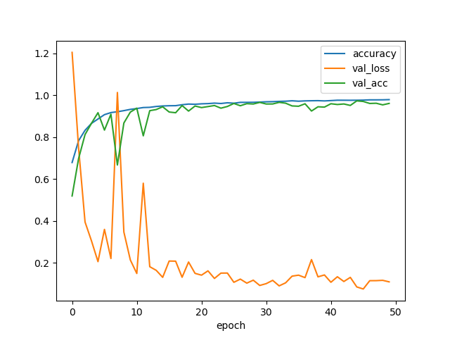
585/585 [==============================] - 252s 431ms/step - loss: 0.0536 - accuracy: 0.9794 - val_loss: 0.1084 - val_accuracy: 0.9613

折线图：

你可能会好奇，为什么没有照片损坏的warning呢？接着往下看吧。

关于检测并删除损坏图片

在陈默涵老师提供了一种方法的基础上，我还用另外两种方法多删除了几十张图片。

先放老师的方法：

用python中的Pillow模块进行损坏图像识别

import os
from PIL import Image

num_skipped = 0
for folder_name in ('Cat', 'Dog'):
    folder_path = os.path.join('PetImages', folder_name)
    for fname in os.listdir(folder_path):
        fpath = os.path.join(folder_path, fname)
        try:
            img = Image.open(fpath)
            img.verify()
        except(IOError, SyntaxError):
            num_skipped += 1
            # Delete corruptep image
            os.remove(fpath)
        finally:
            img.close()

print('Deleted %d images' % num_skipped)

共删除了4张图片。

用python中的imghdr模块进行损坏图像识别

运用 imghdr 模块中的 what() 函数对图片字节数进行读取，若返回空字节 NULL，则判断为损坏图片并删除。

import imghdr
import os

def delect_webp_and_none_type(path):
    i = 0
    for root, dir, file in os.walk(path):

        for name in file:
            target = (os.path.join(root,name))
            result_type = imghdr.what(target)

            if result_type == None:
                # print(target)
                i += 1
                os.remove(target)
    print("Deleted %d images" %i)


if __name__ =='__main__':
    delect_webp_and_none_type("PetImages")

在前述两种方法的基础上，又多删了18张损坏图片。

用python中的subprocess模块进行损坏图像识别

运用 subprocess 模块的 Popen() 方法，启动新进程打开图片，创建一个新的管道，并返回执行子进程的状态，若返回状态非零则表示异常，并以出现异常为标准删除损坏图片。

我们启动新进程打开ImageMagick的Identify图像识别，当识别到损坏图片时将其删除。

import os
from subprocess import Popen, PIPE

folderToCheck = 'PetImages'
fileExtension = '.jpg'

def checkImage(fn):
    proc = Popen(['identify', '-verbose', fn], stdout=PIPE, stderr=PIPE)
    out, err = proc.communicate()
    exitcode = proc.returncode
    return exitcode, out, err

i = 0
for directory, subdirectories, files, in os.walk(folderToCheck):
for file in files:
    if file.endswith(fileExtension):
    filePath = os.path.join(directory, file)
    code, output, error = checkImage(filePath)
    if str(code) !="0" or str(error, "utf-8") != "":
        i += 1
        os.remove(filePath)
        
print("Deleted %d images" %i)

在前述三种方法的基础上，又多删了13张照片。

我并不建议你使用这种方法，因为它会eats你的CPU cycles并会占用你几乎所有内存。如果你对subprocess感兴趣，可以看这里，如果你对ImageMagick感兴趣，可以看这里（谁看到这不感叹一句：What a thoughtful¹ blogger）。

但是，通过这种方法删除照片，几乎能把所有损坏照片删干净

你不禁发出疑问，为什么要删除这么多损坏照片？。原因之一就是减少训练模型时的报错，至于其他原因，Hell knows.

如果你有任何疑问，与我联系。

thoughtful: 贴心的 ↩

Image Classification From Scratch

从零开始深度学习——图像分类

May 08, 2022